|
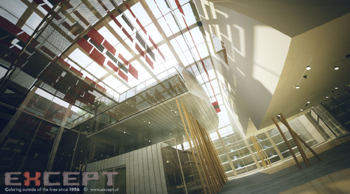 |
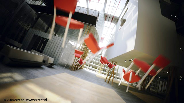
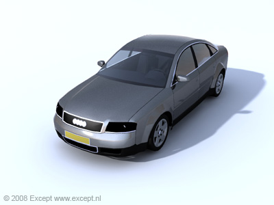
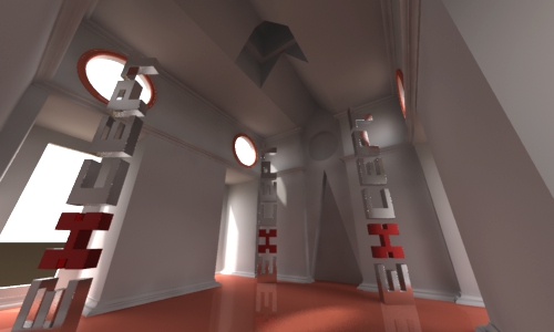
| Except's Wesleyan Museum Rendered using LightWave 9.5 in 8 minutes on a Dual E6600 using Final Gather interpolated radiosity with fairly standard settings (2.0/100 MPS, 200 primary rays, 40 secondary rays, 4 bounce, 300% strength, 50% multiplier) at 1280x700. |
|
LightWave 3D uses two and a half different methods for radiosity calculation. The first one is Monte Carlo, the second Final Gather, and the 'half' is background radiosity. Backdrop radiosity is a special variant of the Monte Carlo method, hence the 'half'.
Each of these three variants can be used with the tick box options, for various uses, speeds and levels of quality and physical accuracy, giving you a broad range of control options to suit your particular needs. It will pay off taking the time to understand the difference of these methods in order to get fast, clean and accurate results. Good radiosity settings will get you fast and smooth results. Bad settings are usually either slow or ugly, or both. Learning how this works is not that hard, and requires only little experimentation with a simple scene, such as the one I'm using for this explanation.
What's new in 9.6?
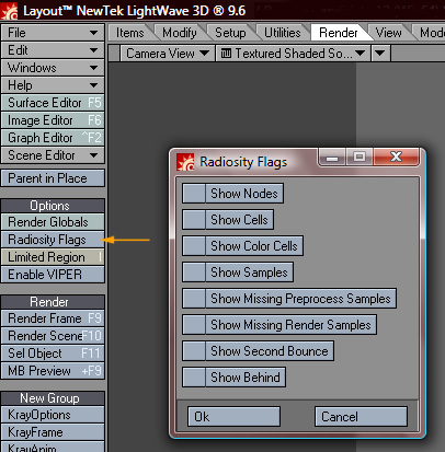
9.5 brought us animated radiosity, per object Gi settings, the GI multiplier, and vastly improved speed and quality. 9.6 on the surface seems to add only a few options, but it again raises the bar for speed and quality. Internally the engine has been tweaked even further, and the 'sweet spot' for your settings has gotten a lot larger. Improvements in the sampling algorithm ensure more consistent performance, and the 'use bumps' and 'use gradients' options expand user control. The 'use bumps' especially is a very powerful feature that solves many issues of the past. Also, the radiosity analysis flags have now been embedded into the interface for easy access, which is a great help to set up your GI perfectly and to understand what is going on under the hood. The RenderQ script was added to provide a single-click cache workflow as well as other great uses.
LightWave 10 improves on the radiosity algorithms and methods explained here, but does not depart from its user operation. The guide is therefore essentially the same for version 9.6 and 10, but in general LightWave version 10 will produce better results.
|
|
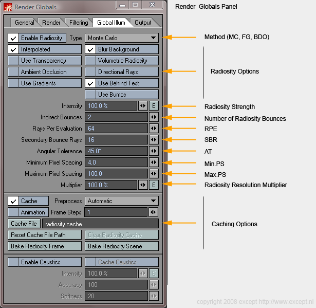
| Setting name |
Short description |
| |
|
| Enable Radiosity |
What it says, it does! Settings will be retained when switching it off or on. |
| Type |
Lets you choose between Monte Carlo, Final Gather and Backdrop only. Available options depend on this setting. |
| |
|
| Radiosity Options: |
|
| Interpolated |
Toggles the Interpolated mode (light cache) for all radiosity modes. This is very important and you should familiarize yourself with this powerful switch. Discussed in detail in the interpolated section. |
| Blur Background |
This only applies to whatever is set in the Backdrop panel (ctrl-f5). It blurs the backdrop for a smoother GI solution, and less noise. |
| Use Transparency |
Changes the way transparent polygons are treated by the radiosity process, also discussed below in the Direct Rays and Use Transparency options. |
| Volumetric Radiosity |
Will cast radiosity from volumetric entities such as hypervoxels, volumetric lights etc. |
| Ambient Occlusion |
Adds the ambient light to the backdrop to use for radiosity purposes, creating an ambient occlusion effect without shaders (good for clay renders). |
| Directional Rays |
Toggles the use of radiosity rays cast by reflection, refraction and other directional effects. This slows rendering down considerably, only use when explicitly needed. Discussed below. |
| Use Gradients |
Toggles the use of weighted GI sample importance. Given sufficient rays this function can result in cleaner and more 'tight' radiosity solutions. Rule of thumb is to leave it off for low RPE's, and turn it on for everything else. I just always leave it on, really. One should note that bump maps are strongly affected by this and may render much more faint with the option turned on. |
Use Behind Test |
The behind test is used to determine whether two samples are on the same plane, to determine whether they should be blended or not. This is important for things like paper lying on a table or stairs. However it does add calculation time per sample, which is negligible for normal scenes, but scenes with many samples suffer, like trees, grass, etc, so you can turn it off with this toggle. |
Use Bumps |
Determines whether bump maps are allowed to generate samples or not. This is useful if you are really making shapes with bump maps, but causes immense amounts of samples to be generated on surfaces with detailed bump maps like rock, water, etc. Leave this off unless you really need to use it. |
| |
|
| Radiosity Controls: |
|
| Intensity |
Scales the intensity of the radiosity solution. Balancing this with the light strength is important for realistic renders. Setting this higher will simulate the effect of extra bounces. |
| Indirect Bounces |
Number of radiosity bounces. More bounces create a more realistic solution, but is slower. After a certain number of bounces the differences are hard to see. For exteriors 3 are usually enough, for interiors between 4 and 8 are usually fine. Too many bounces can also create a bit of a washed out effect. |
| Rays Per Evaluation |
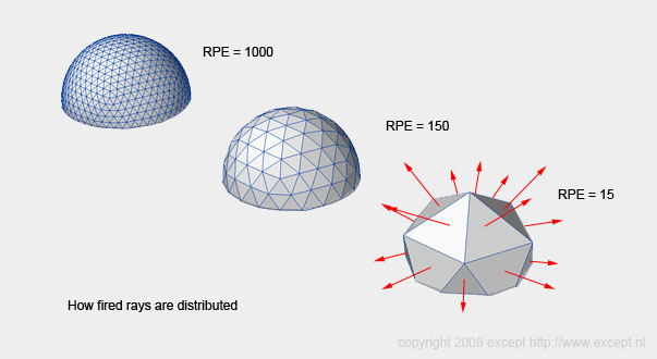
RPE, Number of primary rays cast per evaluation point. These are the rays cast by each primary evaluation point. The evaluation points are distributed as per the diagram below. Try to keep this setting as low as you can, without affecting image quality. Usually 200 is a good starting point. When you need very highly detailed GI in complex scenes this can go up to the 500~1500 range. Going above 1500 is exceptional. (see the troubleshooting section) |
| Secondary Bounce Rays |
SBR, Number of secondary rays cast per primary ray. These inform the primary evaluation point with further shading details. Keeping this low helps speed things up, increasing this can smooth out a blotchy scene where most of the light visible has been bounced a lot rather than direct or first bounce light. Values between 5~10 for exteriors scenes and for interiors 40~80 are good rules of thumb. In extreme multi bounce cases you might need something like 100. More than 200 makes almost no difference, but does slow rendering. Remember that setting this higher casts extra rays per primary ray, so the render hit is exponential. I've only seen an example where this needed to be higher than 200 once, which was the dreaded kitchen scene. (see the troubleshooting section) |
| Angular Tolerance |
Defines the density of placement of radiosity samples for curved surfaces (see diagram below). A higher degree setting here creates less samples on the curved surfaces, and lower more. Internally the cutoff is 10 degrees, so setting it lower than that always makes it 10 internally. Setting the AT higher than also 45 degrees turns OFF the behind test, despite the separate toggle. You can set this per object using the per-object GI settings, which is useful for trees, plants and grass and so on, as they will eat up samples like mad if you don't set their AT high (60~90 degrees) |
| Minimum Pixel Spacing |
Min.PS, minimum spacing of radiosity samples between output resolution pixels. |
| Maximum Pixel Spacing |
Max.PS, maximum spacing of radiosity samples between output resolution pixels |
| Multiplier |
Scales the output resolution of the camera internally to compute the GI at lower/higher resolution. This is a very powerful feature, as in most cases the radiosity solution does not need to be as defined as the final frame output. Radiosity is a subtle effect and can be upsampled quite well. So, for example, you're rendering a 800x400 frame, setting this to 50% will render the radiosity at 400x200 pixels, and then scale it up the fit the mode. Setting this too low will end up giving you shading artifacts.
Note: Leave this at 100% for animated GI! |
| |
|
| Cache Controls (also below): |
|
| Cache Checkbox |
Switches the use of caching on and off. Settings are retained when switched off. |
| Preprocess |
Changes the way the GI preprocessing is handled and stored. Choices are Automatic, Always, Never and Locked (see above). Default is Automatic. |
| Animation checkbox |
Switches on the animated cache functionality. This only works when Monte Carlo or Backdrop Only has been set as the radiosity mode, since Final Gather does not support it. |
| Frame Step |
Defines the frame step for the radiosity preprocessing. This is useful to spread out the calculations over an animation rather than doing each frame. With slow camera movements this can easily be set to high frame numbers. Ideally one would want only small overlap between calculated frames, to prevent overhead. |
| Cache File Path |
Hitting this allows you to set a path for the cache file. A name is automatically filled out if you don't set one manually. |
| Reset Cache File Path |
Resets the cache file path to the default location. |
| Clear Radiosity Cache |
Deletes the cache file, but the path will stay the same. |
| Bake Radiosity Frame |
Calculates (preprocesses) the GI of the current frame and stores it in the cache file |
| Bake Radiosity Scene |
Calculates (preprocesses) the GI of the entire scene as defined in the frame range & Cache Frame Step |
|
|
The term for radiosity calculation in LightWave is radiosity preprocessing. We can discuss it in terms of two stages, although in reality there is more going on, but this is all you need to know to deal with it effectively. Below these two stages are explained.
|
When using the interpolated option, which will be in 99% of all cases, LightWave places samples in the scene depending on the geometry detected. This process is explained here. |
|
Min / Max MPS
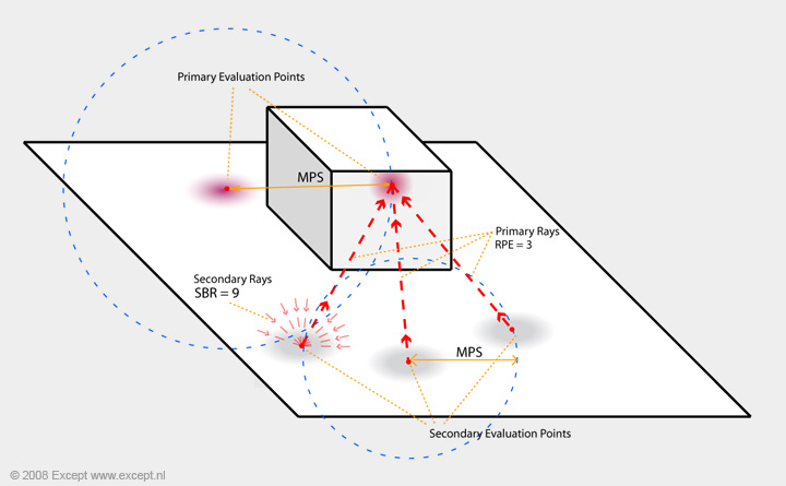
Samples are placed close to geometry changes and more widely spread on large even surfaces. The major setting for sample placement is the Minimum and Maximum Pixel Spacing (MPS) setting. This defines the range that samples are allowed to be apart in terms of output resolution of the camera. While the samples are thus placed in relation to the camera resolution, the samples are attached to geometry. It's like shooting sample points through the camera after which the stick to whatever they were shot at.
This process makes primary evaluation points. In stage II below the rays are shot, but the primary rays (those that were shot from the primary evaluation points) also generate evaluation points if they hit a spot where there is no other evaluation point close enough. These secondary evaluation points are also controlled by the MPS settings. The secondary rays shot from the secondary points do not generate evaluation points. They sample what they hit, pass down the value and then the sample is discarded.
The below diagram shows two primary evaluation points (purple) and three secondary ones (gray). The secondary evaluation points inform the primary ones through the primary rays (RPE), and they in turn get their illumination values from the secondary rays (SBR). The blue circles are planar to the camera's field of view and represent the MPS ranges.
The below image shows the relationship between min. PS and max. PS. The green dots are evaluation points (both primary and secondary). The one on the left has a large range (1.0-100 mps) and the one on the right a small range (30.0 - 60.0 MPS). You can see that when min and max come closer together the samples start representing more of a grid in relation to the camera. Setting them further apart allows samples to crowd around areas of higher importance and large even areas to have only a sparse distribution. But don't overdo it, 0.5-500 would be an unlikely setting for any kind of situation. min. PS is often happy anywhere between 1.0~4.0, and max MPS between 40.0~200.0. Use the display of samples to see what's going on (see end of this guide) but you can also defer it from the preview which shows unblended shading of samples, thus you can see where things crowd. (btw these images were scaled, so their pixel distances don't match the figures, but they are correct in relation to one another) 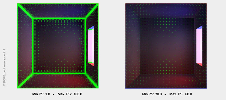
|
| Angular Tolerance |
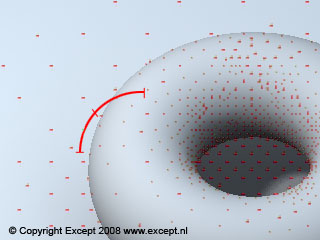
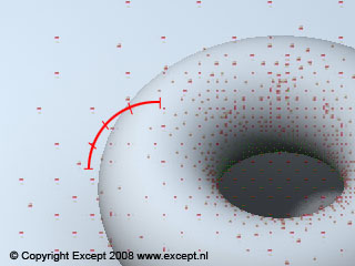
Angular Tolerance is the second setting for sample placement and it forever confuses everyone. What it does is control the amount of samples minimally placed on curved surfaces. It works in a similar fashion as the smoothing angle in surface editor. Below two renders which show sample placement, one with the default of 45 degrees, and one with 20 degrees, the smallest allowable angle. You can see that the sample density on the flat plane has not changed, but the curved outside area of Hank the Donut has more samples in the 20 degree image than in the 45 degree image. The density of inner samples is due to the light bouncing around there, not due to the angular tolerance.
 |
 |
| Hank showing samples with an AT of 46 degrees |
Hank showing samples with an AT of 20 degrees |
|
|
Once all the samples are placed, each sample (evaluation point) shoots a number of rays equivalent to the RPE setting. These rays then hit surfaces, and additional sample points are created (as described above), and from these the amount of rays defined by the SBR setting are shot if the GI bounces are set to more than 1. These new rays then hit points which in turn cast another single ray, and this continues until the amount of bounces are satisfied.
|
|
| |
RPE
Each ray shoots the amount of rays defined in the 'Rays Per Evaluation' setting, according to a hemisphere. The distribution of rays shot can be seen in the diagram below.
Once the preprocessing is done, rendering is commenced. This does not mean the radiosity process is at an end. During rendering places which were unseen during preprocessing can become seen due to subpixel sampling by anti-aliasing or Motion Blur. These samples are then added and calculated as well. Thus a the normal pass of a render with radiosity can be slower than a normal pass of a render without. If you use caching read up on the caching options on how the storing of these various types of samples can be handled in the cache file.
|
|
There are three 'modes' of radiosity in Lightwave. This section discusses their differences and application.
In short:
Monte Carlo is the slowest but most accurate way of radiosity calculation, FG is a method taking a few shortcuts resulting is faster calculation at times.. Backdrop Only is a special mode of MC radiosity that only casts light from the backdrop and self illuminating surfaces, which is handy for fast outdoor scenes.
All modes can be used in interpolated mode and not. This makes a very big difference, and changes the operation of the mode significantly. Because this is so important, interpolated mode will be discussed first, and applies to all three methods.
|
Interpolated mode is the name of Lw's advanced GI method. It only calculates the radiosity where samples are placed, not for every pixel of the final image. This saves tremendous amounts of render time. This mode makes the radiosity in LW biased, rather than un-biased (these are technical terms used to define render methods).
Interpolated mode uses the Max. and Min. PS settings in conjunction with the AT setting to determine sample placement as described above. It then fires the amount of rays set by the RPE setting for each of these spots to see what shade they should be, and averages (interpolates) the area in between the evaluation spots to allow for a smooth result. This potentially eliminates a large amount of evaluation spots, as radiosity does not need to be computed for each pixel on the surface. Good settings are required to prevent splotching when using interpolation. The more detail in your scene, the more memory it will consume, as it has to remember all of its evaluation points, interpolate them, etc. This mode renders progressively, which means you see the entire image in rough very quickly, and LW refines the image progressively. This is a great way to preview all scenes that use radiosity, and you get an impression of your scene very quickly. |
|
| |
Min/Max PS:
Sets the minimum and maximum amount of pixels each evaluation point will be apart. Imagine looking into a room, the evaluation points will be closer together near to the camera and further apart far into the room. Remember that if you change your image resolution, you need to change the Min/max PS setting accordingly! You don't want to render with a Min/max PS of 1.0/50 with a 5000x3500 image, as you will surely run out of memory. If you have a render set up that you like and want to increase the resolution, either use the resolution multiplier in the camera settings, as it will internally multiply the Min/max PS settings, or increase the Min/max PS settings with the same factor as you increased the resolution.
Strategy:
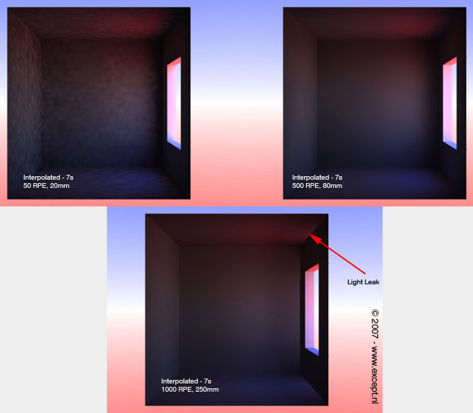
The calculation time is a balance between Min/max PS and RPE. Too low Min/Max PS, and your render will be slow. For each point, the amount of rays set by the RPE will be fired. When you have a good MPS settings, the RPE setting becomes less critical. Adaptive sampling does nothing for Interpolated radiosity to improve it, once the settings are set, there's no way to improve its quality. Below three examples of interpolated radiosity (FG). The left render has too little rays fired, resulting in splotches, and the bottom render has too high a Min/max PS resulting in light leaks and washed out colors. The right one has a good balance between them. Notice the render times of all three are equal.
Use in animations:
Interpolation is an approximation of the radiosity in a scene. Because of this, small errors occur that cannot be seen by the eye, but if repeated on each frame in an animation, it will result in flicker. A solution for this is to 'cache' the radiosity. The samples and their illumination are stored on disk and each subsequent frame they are read back in so that they don't jump around and their shading is identical to the frame before. Also, doing this they do not need to be calculated again so you can achieve huge speed gains by using caching. Caching is discussed below separately.
|
|
This is the considered the default GI method. It is very accurate, and takes few shortcuts, making it suitable for most purposes. In used without interpolation, it fires sample rays for each pixel in the scene (basically the MPS is 1.0/1.0 and each pixel is an evaluation point). It is a physically accurate method, and deals with transparency properly by maintaining the angle and color of the penetrating rays. It is used by various engineering packages to calculate light, but also fluid, thermal dynamics and so on. Monte Carlo can be considered a brute-force method, although it's a bit smarter than that. Used without interpolation its solution always resolves into more or less grain, never splotches or leaks. Non-interpolated Monte Carlo uses very little memory to operate as its operation doesn't depend on or interacts with other samples much. Monte Carlo can therefore be faster than other methods if the memory requirements for these other methods are high. (Wikipedia Link for Monte Carlo)
If used without interpolation, Monte carlo is resampled when adaptive sampling from the Anti Aliassing settings is executed. A good strategy is thus to use a very low amount of RPE for MC and to let the AS system determine where it is too grainy and add extra samples.
Monte Carlo, like the other GI methods, is generally used with the 'interpolation' option on. If the 'use transparency' and 'use direct rays' options are off, MC is usually about the same speed as FG, if the scene has only a few lights. The more lights are added, the faster FG will be over MC.
You might use MC without interpolation because it saves memory, does not require caching, and removes the chance of splotching, flickering and bad GI shading. You pay for this by much higher render times. |
|
Strategy Non-interpolated MC:
The result of monte carlo when improperly set is never splotches, but always noise. Getting a noiseless MC render can take quite a bit of time, and requires the right amount of rays to be set (the only setting it has), so it works well in combination with the new Adaptive sampling system, which will detect noise above its tolerance level and shoot extra samples to remove them. Setting the rays to very high is therefore very silly, and will guarantee you will be rendering much too long than necessary. Set them low and let the AS system take care of it. There might be instances you want to choose MC over other methods for animation, for instance for exteriors, it's sometimes even faster, or for very complex scenes where the memory usage of other methods causes it to slow down a lot.
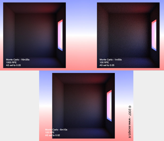
The below example shows three non-interpolated MC renders with differing numbers of rays. As you can see, the low amount of rays causes more grain (up to the 0.05 tolerance I set for the AS system)... Using AS for MC is very valuable, because a low ray render will be augmented by the AS system, therefore only using up as many samples as needed, and the high ray render will be wasting time on rendering areas that were smooth enough as it was. I added one render (bottom) to show the grainyness that would result from a AS 0.02 render instead of the AS 0.05 render. As you can see, it looks nearly identical to the 1000 rays MC render, except that it is much faster.
If at all possible, use interpolated with MC, as it will greatly improve speed and remove any grain.
In the following image, you can see why you would use Monte Carlo over FG or BDO. In the box a dielectric lens is placed, and a bright box a little further away. The MC method refracts the light correctly, bounces the red and blue light properly and delivers a believable image. Final Gather does not take in account color or directionality of samples, and thus mumbles the colors and does for the refraction and light transport of the lens, but it is much faster. This results in a render without caustics (the focused spot on the wall where the lens focused the light in the MC render). The Backdrop Only render shows that it uses the MC method (caustics are generated), but lacks bounces to make it useful in this situation. 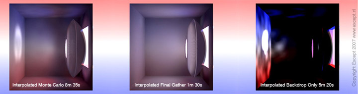
|
|
The second algorithm to calculate radiosity in Lightwave 3D is Final Gather. This is provided as an alternative to Monte Carlo, and is somewhat faster, at the price of less physical accuracy (see bottom of page). Its speed gain increases when there are more lights present. FOr few lights, and not using the 'use direct' and 'use transparency' options, the speed difference between Mc and Fg are negligible, but MC has considerable nicer blending and smoothness. As with MC, FG is usually used in interpolated mode. Not using Fg in interpolated mode does not give it the same characteristics as MC, as it will still flicker in animation. The reason for using non-interpolated FG is therefore hardly worth defending.
First, a rough and very fast pass is performed (which can be cached), for all the secondary rays. Because secondary bounces are usually very faint, FG shoots very little rays and interpolates between them for these secondary light effects, speeding up the calculation enormously, especially with large amounts of bounces. This is why non-interpolated FG still uses the interpolation settings MPS/AT even when not interpolated. Because it stores data on the secondary rays in world space, FG uses more memory than MC does. After this a pass is performed to fire the primary sample rays per pixel. This pass resembles the MC method in appearance and might produce noise.
Final Gather also gains speed by not calculating the directionality of rays. Thus, all surfaces radiate in a diffuse manner. It is important to account for this when using windows through which daylight enters. It will not be correct and the render times will be longer than necessary. For this the 'use transparency' and 'Direct Rays' options were added. When both are off, transparent polygons are completely ignored, and they do not affect FG calculations. If you want to use transparency with FG, using the FG rays, set 'Direct Rays' to on. By doing this, you might find that the directionality and colors of the rays gets lost, but in many cases it can be useful. If color and directionality is important to you, use the 'use transparency' and 'directional rays' options together, then FG will use MC to trace through transparency and thus be correct. I twill be slow though, but faster than straight MC. A separate section goes into more detail about these switches below. |
|
| |
Strategy:
Because the most time for an FG render is spent in the second pass , you want to keep the RPE low, and let the AS system take care of the noise, as with the MC method and any other stochastic method used in Lightwave 3D (such as the reflection and refraction blurring, Photo real motion blur and DOF).
FG is potentially very effective for scenes with much detail, but take too long for MC. The first pass of FG can be cached so there's a performance gain each frame for FG versus MC. The speed gain will depend on the amount of secondary bounces (which are cached) versus the primary ones (which are not). If you're using non-interpolated FG the trick is to really crank up the settings for the first quick pass (MPS, tolerance and SBR), and keep the RPE low, while using AS to take away the noise.
However, it makes much more sense to use FG with the interpolated option. I have found very few instances when I would use FG without it. It greatly improves speed, as well as removing any kind of noise present.
|
|
This method is based on the Monte Carlo algorithm. What is does differently than plain MC is that it only fires radiosity rays from the background and self-illuminating geometry. It is essentially a non-bounced radiosity method. It's therefore really fast and very useful for outdoor scenes that need some quick environment illumination, like from an HDRI or a background gradient. It also does not use much memory. Great for those clay look renders in white rooms. This can also be interpolated. |
 |
| Typical use of Backdrop Only radiosity, an exterior scene with not too much bouncing off surfaces. Rendered in 16 seconds on a Q9450 at 640x480. |
|
|
|
These options were added in Lightwave 9.5 and allows you to switch off the radiosity rays cast by reflection, refraction, specularity, transparency and other directional (non-diffuse) sources. They are both off by default. Keeping this off can cut your radiosity time in half (but will NOT affect the normal render pass), but it should be used with care, as it might disable the subtle effects you might just be looking for. However, the speed gain is significant and in most cases, if you do not need it, or can organize your scene so that you don't need it, it will benefit you greatly to turn it off.
Directional Rays are all rays cast from surfaces that have some directional property to it. Examples are antistrophic surfaces, bump maps and sub surface scattering. If you wish to focus light through a lens as some of the above examples do, you need this to be on.
This is a list of exactly what happens in relation to the two settings:
| Directional Rays off Use Transparency off |
All radiosity modes will not compute directional rays (anisotropy, bump map effects, refraction, etc), and will treat transparent polygons as if they're not there. |
| Directional Rays on Use Transparency off |
MC and FG will use all directional effects and treat transparent polygons as if they're not there. |
| Directional rays on Use Transparency On |
Mc will compute all effects including transparency accurately. FG will do something fancy: trace all rays with FG but switch to MC when hitting transparent polygons, to ensure that they are not treated as diffuse, and to catch color and so on. |
| Directional rays off Use Transparency on |
All radiosity modes will not compute directional rays (anisotropy, bump map effects, refraction, etc), and will trace light through 'simple' transparent surfaces (no refraction, no nodal). Complex transparent surfaces will become opaque. |
Use transparency will make LightWave trace through transparency affecting the rays. This has a render hit but is sometimes necessary. With it off, transparent polygons will be treated as if they are not there at all, speeding up the process. Turning it on will make MC see transparency polygons, and it will make FG trace through transparent polygons using the MC method with directional rays set to on, and using FG when set to off.
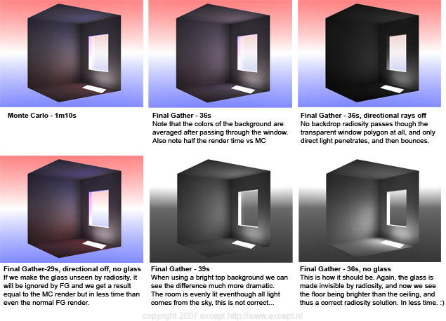
In order to better understand the 'use transparency' option, take a look at the following diagram, describing the effects of a transparent polygon (red) being hit by a directional light source for Monte Carlo, and Final Gather with directional rays off. If directional rays are on FG will behave much the same way MC would when tracing transparent polygons:
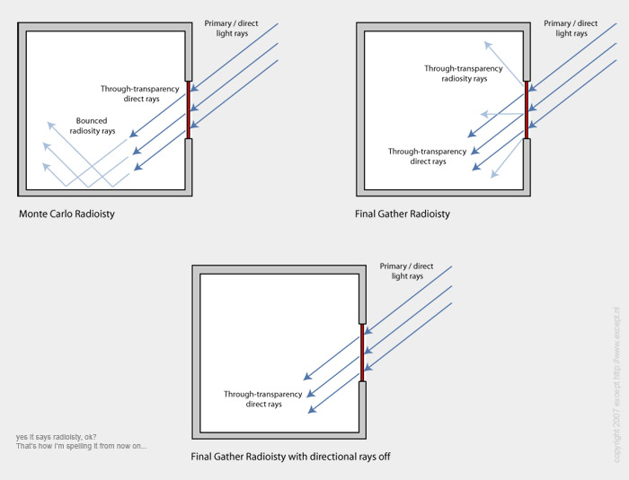
This might seem confusing at first, but it is important to remember the differences between the Monte Carlo and Final Gather algorithms. The first image shows what the ideal situation is, which is what Monte Carlo does. The light penetrates the transparent polygon and continues on its way in its original direction, bouncing around further along the trajectory.
The second image shows what happens when Final Gather rays hit transparent polygons. Since Final gather does not take directionality of rays into account, when a surface is hit, no matter what surface, the subsequent radiosity rays are cast in a diffuse manner, and without color cast. This proves to be a problem with transparent surfaces such as windows, where the directionality of the radiosity is lost, and a non-accurate solution will result. You can therefore enable 'Directional rays' so LightWave will use MC to trace through the glass, slowing it down but providing accurate shading even though the FG method does not allow it natively.
The below examples have 'Use transparency' set to on.
|
Why Caching?
Caching is used for radiosity processes for two main reasons:
- To speed up rendering by saving already calculated data and reusing it when the data can be applied
- To make sure animations don't flicker.
Without caching animations with interpolated radiosity will flicker due to the slight variations in shading for each newly calculated radiosity solution, and it's extremely hard to get rid of this. Before caching the only way to use GI and render animations without flicker was to use non-interpolated Monte Carlo which is very slow and usually this disqualified using radiosity for animations, making people resort to setting up elaborate lighting rigs to simulate radiosity without actually using it. These rigs still come in handy sometimes, but with the speed and caching options of radiosity in LightWave today, using radiosity is usually both faster and easier to setup as well as faster to render.
There are two entirely different modes of caching in LightWave. One is called the static cache, which is the default, and the other the animated cache. They work quite differently and have different applications. Expecting one to work like the other is the source of many wasted computation hours and frustrations, so understand the process and properties well for each. There are various work flows possible to suit your needs, and it is extremely flexible in its application.
How the information is stored
Caching stores some but not all of the information associated with these calculations which are called 'preprocessing' in LightWave (the red progress bar in the render status window). Depending on the cached mode, different information will be stored. The static cache (when the animation checkbox is off) stores the evaluation points including their shading. Because the shading is stored it cannot change and any changes in light or object movement will not be reflected in the solution. Sometimes this is not a problem, but if you have animation where other things move other than the camera, you will have to use animated caching. Animated caching does not store the shading information, only the location of the sample points. This means the calculation of the cache is much faster than that of the static cache, but the GI is recalculated each frame, thus slower, since it has to recalculate the shading for each frame all over. This does however allow you to use radiosity and animate nearly everything, lights, objects, and so on. There are some restrictions to using this, which are summed up further along.
The radiosity process as explained above details two stages: the placement of samples and the casting of rays to collect information for the shading of those samples. In the interpolated modes the samples are then interpolated to get a smooth result. For each preprocessed frame information of the radiosity process is then added to the cache file on disk. The radiosity process works in full 3D space, and that information is also stored that way. The samples are really lying on top of the geometry they are shading. This means that it is not associated with anything other than the geometry it is affecting, and not with a particular camera or surface. A cache can be created with one camera and rendered with another. As long as all the areas visible to the second camera have been preprocessed, it should work just fine. This also means that during the calculation of a cache LightWave can already make use of the cache to speed up rendering. Let's say your camera moves half a view angle after the calculation of the first frame to calculate the cache for the second frame, half of the space that camera sees has already been processed therefore can be loaded from disk. LightWave handles this automatically and you do not need to remember what has been stored or not. If you accidentally try to store an area which has already been done, LightWave still preprocesses it, but by reusing the data already on disk will be really fast thus not penalize you with a lengthy unnecessary render.
The process:
First a cache location and file has to be set. The file will be automatically created when it does not exist. Then there are two ways to go about making a cache:
- Render the scene and have each frame's radiosity information stored to disk
- Bake the radiosity of the scene and render the scene afterwards
Some of this is personal preference, but there are some differences to be aware of. The first method tends to render slightly faster as some processes in the second method are redundant. But even for big scenes those differences are small. However you do have a two-step process in between which the computer might be sitting idle because it requires user intervention to start the render phase once the scene has been baked. The second option has its main application for network rendering. Instead of rendering the frames immediately on one machine, one often wants to use a render farm. You 'bake' the scene, which means as much as generating just the radiosity cache and not render, and then have all the computers in the network use that stored cache to create flicker free radiosity animation over the network.
Preprocessing can be done in various ways, depending on your use. Normally preprocessing is set to Auto and this works for most situations. It should be noted that LWSN nodes always use the 'locked' method regardless to what the scene is set to. Here's a description of the various preprocessing modes:
| Preprocessing mode: |
Description |
| Automatic |
Automatic preprocesses each frame in compliance with the cache Frame Step setting, and stores all the information available. It remembers which frame has already been stored, and will skip preprocessing of these frames and just load the solution if it encounters them. It will make sure that frames in between the set Frame Step are also not preprocessed. |
| Always |
Forces LightWave to always preprocess a frame regardless of it already having bee processed before. This is necessary when you have 5 cameras in a room pointed at different directions and you want to bake to the cache from each one without actually going through different frames. If you use Automatic in this case, LightWave will detect that the frame has already been processed and skip it, however you are using a different camera which sees different things so you'll have to use 'Always' to force it anyway. It's also necessary when baking a few single frames in between the frame step interval to enrich the cache where it's necessary. |
| Never |
Uses the cache saved to disk and never preprocesses it. This is useful when you have a nice cache of a space and do not feel it needs further refinement. You can then extend the frame range and it will never preprocess. However, samples are still generated in previously unseen areas due to spatial effects of AA, Motion blur and others during normal rendering. These samples are still stored to disk with this setting, and reused for other frames. |
| Locked |
This mode is much like 'Never' except that it does not store the samples it finds during rendering to disk. It does compute them to make sure there are no black holes or ugly unseen areas and artefacting, but it does not touch the cache file at all. This is a good setting for a scene where the cache has been carefully constructed and you want no scene to mess with it, just use it. This is the mode LWSN operates in, as they are not allowed to write to the cache file. |
The options
Below the different options available and a description of their use and function
| Option: |
Description: |
| Cache Checkbox |
Switches the use of caching on and off. Settings are retained when switched off. |
| Preprocess |
Changes the way the GI preprocessing is handled and stored. Choices are Automatic, Always, Never and Locked (see above). Default is Automatic. |
| Animation checkbox |
Switches on the animated cache functionality. This only works when Monte Carlo or Backdrop Only has been set as the radiosity mode, since Final Gather does not support it. |
| Frame Step |
Defines the frame step for the radiosity preprocessing. This is useful to spread out the calculations over an animation rather than doing each frame. With slow camera movements this can easily be set to high frame numbers. Ideally one would want only small overlap between calculated frames, to prevent overhead. |
| Cache File Path |
Hitting this allows you to set a path for the cache file. A name is automatically filled out if you don't set one manually. |
| Reset Cache File Path |
Resets the cache file path to the default location. |
| Clear Radiosity Cache |
Deletes the cache file, but the path will stay the same. |
| Bake Radiosity Frame |
Calculates (preprocesses) the GI of the current frame and stores it in the cache file |
| Bake Radiosity Scene |
Calculates (preprocesses) the GI of the entire scene as defined in the frame range & Cache Frame Step |
The actual working of the animated cache has been described above. However, there are some things you want to consider when you work with it a lot, or in specific scenes. First, you won't save much render time with it like the static cache does. It's really only preventing flicker. That's usually fine as LW's radiosity is really fast. There are also several circumstances in which the animated GI does not work well. Here's the list so far:
- Deformed objects (creates millions of sample points, renders very slow, and eventually might run out of memory)
- Volumetric plug-ins (HD Instance)
- Intersecting objects can create light artifacts on the intersection
- Small very bright luminous objects can cause flickering due to the rays being too dispersed creating too large a variance per shading point
- Moving shadows do not generate extra sample points, thus can look a bit ragged. Increase sample density if possible.
- Do not use the GI resolution multiplier with animated GI. It causes increasingly longer render times and possible flicker.
Truly understanding how the cache system works might allow you to understand these items more, but also might make you aware of potential problems. If your animated cache (to a limited degree this is valid for the static cache as well, but there it isn't as noticeable) goes increasingly slower... eg a long animation takes four times as long per frame after baking than without a baked solution. This would seem like a bug, but it actually makes a lot of sense, and it works as it's supposed to, and you can control for this as well.
The below scene had this problem at some point.
Understanding the caching process you can see why this happens. When baking, it places sample points only. However, it does so for the entire animation. If you zoom into a wall or objects turn, swivel and reveal parts of the scene that was previously unseen, more sample points are generated. On some complex objects with a lot of irregular geometry, or very complex scenes, these sample points might start to accumulate a fair bit (see example image below). So, after the scene bake, every frame has considerably more sample points than rendering a direct frame.
There are several ways you can solve this.
- You can increase the MPS settings (example: 1.0-50.0 to 3.0-200 perhaps). While for a single frame this might be ugly, once the bake is done, it likely has plenty of sample points accumulated.
- You can bake using a frame step larger than one (my preferred method). For slow movements you can increase this quite a bit, as not a whole lot is revealed in the meantime. I have had scenes where this was set at 20. this means new sample points will only be generated every 20th frame, resulting in much less cluttering. Setting this too high, however, leads to flickering, because sample points are missing where they are needed, and LW fills them in on the fly to prevent gaps. So be careful, run a test if possible.
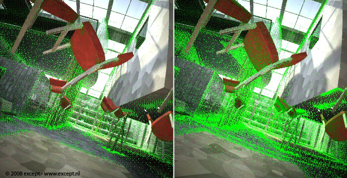 |
| Render showing sample points without baking |
Render showing sample points after baking 200 frames |
|
Using RenderQ
The disk cache always needs to be created with a single computer. This part of the process cannot be distributed among a network of computers since each frame is highly dependent on another. However, since it's always recommended to bake the scene first prior to rendering it, a tool called RenderQ helps when using a single machine. It's like a tiny scene render manager that allows you to set up various scenes to render in a 'play list' of sorts, and then performs them. It has a special switch for baking in the bottom right corner. When this is enabled, all the scenes that are added will bake the GI first, then reload and render the scene. Very handy!
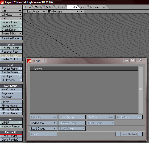 |
The RenderQ panel
You need to use the 'close RenderQ' button to stop the panel from popping up every time you start LW. |
|
Cache Tips
There are many ways to use the cache. Here are some tips that might indicate some uses, and some tips:
- Bake a cache of a scene, then set the preprocessing to 'locked' and now play with the colors and surfaces of the scene. You see that you can still change them, except that their color cast does not update. Usually color cast and bleed is subtle and for previewing is not necessary. This is a great way to discuss material selections with a client without doing a lengthy radiosity render over and over again. Just use the cache and once selections have been defined, re-render the cache to make sure all color bleeds and casts are performed using the correct surfaces.
- Do not use the animated radiosity when you do not need it. Firstly, it has more restrictions, and second, illumination is not stored, only sample placement, thus you might not have much speed gain compared to normal non-cached rendering.
- The cache frame step is remembered once a cache has been baked, even though you change it, which can be a bit confusing, as it won't actually perform that change.
- Even when doing random test renders, keep the cache on. You can always hit 'clear cache' to reset it fast, and it does not cost any render time to save the cache file.
- Cache data is saved to the cache even when a render is aborted, therefore you can pick it up where you left off, and it will reuse the data that was already rendered. This does mean you'll have to clear the cache if you make a significant change to your scene before rendering again or it might use incorrect cache data.
- If you have very highly irregular objects in your scene, it might be that the cache system keeps adding new samples because areas are per frame seen that were unseen, like grass, trees and so on. The cache may get choked, rendering goes increasingly slower and eventually might become unworkable. In these cases, reduce the problems by using high Angular Tolerance, and make sure 'use bumps is off. If that's not enough bake out just a few frames of the animation, enough to have full coverage of all large objects, and then set preprocessing to 'never'. That works well and you'll get a constant render time without choking. The samples will still be generated but discarded afterwards, and thus not create congestion further down. You do risk flickering here, so make sure you do a test run.
|
You have this one scene where you just can't get rid of the splotchies, and it's driving you mad. We know this scene. We've got one too. Juggling values is then bound to happen with many tests and many results. I've done this personally many times and the knowledge I gained from this is all over this guide. However, I wanted to re-iterate some important concepts. This test scene can be downloaded below.
Undefined or crude GI: MPS setting
First thing to set right is your MPS range. Depending on the scene you might want to lower your max-value. This forces more samples to be placed in the scene. This will also slow down rendering. Setting this too low does NOT lead to splotchies or artifacts usually, it will lead to undefined radiosity. The example below (click on it) shows the difference between a decent and a too low MPS setting. Note that it is still smooth. A very high RPE setting was used to discard this as a factor.
 |
 |
| 3000r - 100s - 10.0-200.0 MPS: 52s |
3000r - 100s - 1.0-40.0 MPS: 5m20s |
Splotchies: RPE and SBR setting
If you're getting splotchies, first thing to do is crank up the primary rays amount. Try doubling it first, then continue on. Or if you have enough time, and want to be sure, choose something between 1000-2000 for complex interior scenes. This does not necessarily render slow, but of course it'll affect render time. If this doesn't work, increase SBR, but if you're going higher than 100 with SBR, consider other causes for the problem. Modeling errors can give faults as well, and so can incompatible plugins.
 |
 |
| 200rpe - 100sbr - 1.0-100.0 MPS: 56s |
1000rpe - 100sbr - 1.0-100.0 MPS: 2m16s |
Remember that SBR only has very subtle influence over the scene and that it need not be increased when RPE is increased. In fact, sometimes a value as low as 10 cannot be distinguished from much higher ones, except in render time. The right render of the above example takes 2 minutes and 16 seconds, but when I drop the SBR to 20, only a tiny change in the splotchies is visible, while the render time drops by almost a minute. You can invest this render time in a higher RPE for a much smoother result.
 |
| 1000rpe - 20sbr - 1.0-100.0 MPS: 1m34s |
Optimize: Multiplier setting
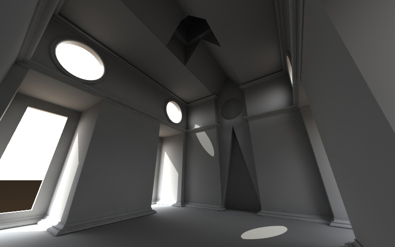
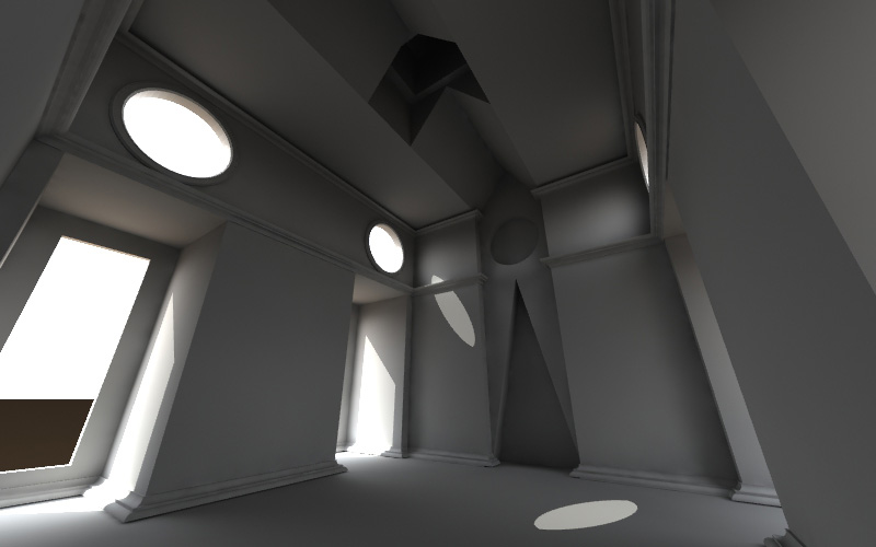
So you have found settings that make your render look good, but it renders too slow for you still... we all want faster and faster, don't we? Okay, Multiplier to the rescue. The multiplier calculates GI with the same settings but scaled down in resolution compared to the camera resolution. So, if your camera is set to 1024x768, and your multiplier to 50%, your GI will be calculated at 512x384. This can reduce render time by 4 (at 50%), while sometimes hardly sacrificing quality. In the case of this chapel, I can crank up the RPE to 3000, and the MPS to 1.0-40, and get a render time that's over 5 minutes. When I then set the multiplier to 50%, I get virtually the same result in less than 2 minutes.
|
 |
| 3000r - 100s - 1.0-40.0 MPS @ 100% : 5m20s |
3000r - 100s - 1.0-40.0 MPS @ 50%: 1m50s |
Lots of trees!
Specific applications require some other settings to be taken into account. One example is objects which are highly irregular, like plants, trees and grass. They eat up samples like crazy and the safety built into LW to have overlapping polygons not blend together accidentally will start to cost a lot in terms of render time. For these objects you want to disable the 'Behind Test', and make sure they have a high Angular Tolerance. Lucky for us, the AT setting controls both. Setting it to 46 degrees or above disables the behind test. Use the per-object GI settings in object properties if you don't wish to do this for all objects in the scene (but that's usually okay).
Test Scene
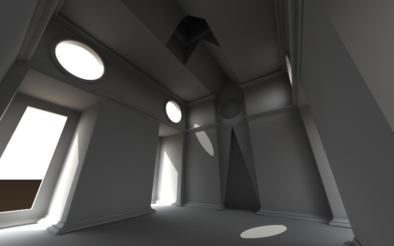
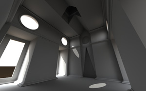
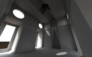
For your enjoyment I have provided the above test scene, with some additions. It's a useful scene to experiment with various settings and effects with quick render times. It's a demanding scene due to the thin detail of the wall skirting, and the completely indirectly lighted interior. The radiosity settings reflect a nice balance between speed and accuracy, and this scene renders at this resolution in 25 seconds on a Quad Core2 at 2,66Ghz. This image is re-exposed at 65% black point. Download the scene here.
 |
| GI Test Chapel scene, MC int., R 400, S 50, AT 50, Min 1.0, Max 100, M 50% |
|
|
The radiosity flags are diagnostic tools designed to show some of the internal workings of the render engine, for analysis, troubleshooting and learning reasons. A list of these is provided below, and an example render for each provided. The caching section above already uses one mode to clarify some operations.
You can combine these flags to show the data you need for analysis.
Some examples:
|
|
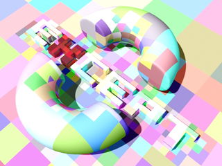
| "Nodes" - Octree nodes as random colors |
"Cells" - Nearest sample cell shade |
| |
|
|
|
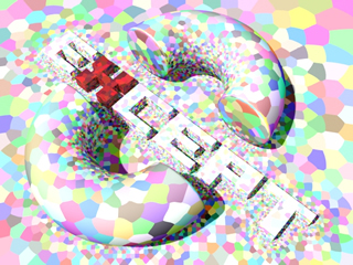
| "Color Cells" - Nearest sample cell shade with random colors |
"Samples" - Sample locations (green) |
| |
|
|
|
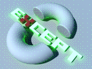
| "Missing Preprocess" - Shows the samples which were missing during preprocessing (cyan) |
"Missing Render Samples" - Shows the samples which were missing during rendering (purple, hard to see) |
| |
|
|
|
| "Second Bounce" - Shows the second bounce cells |
"Behind" - Shows the behind test operation |
|
| Links & other tutorials |
If this tutorial proves especially handy for you, would like to support the creation of more of these tutorials and new developments, or would just like to express your thanks, you can make a donation by clicking on the following button, or alternatively just send me an email.
Go To Presentation Resources page
Go to Except Web site
This guide is Copyright 2008 Except Design, and written by Tom Bosschaert. Nothing from this website can be copied, transferred, published or distributed in any way without prior written consent from the author.
|
|